Building Materialized Views for Predictable Analytics on Apache Pinot

In a real-time analytics system, performance is only one part of the problem. Operators need the cluster to stay healthy when the same expensive aggregation arrives from a dozen dashboards at once. Users need to know how fresh the data is — without standing up a separate ETL pipeline for every new metric. Materialized Views are how we make that contract first-class inside Pinot — owned, refreshed, and applied to queries by the engine itself.

Why Pinot needed materialized views

Three scenarios kept showing up in our on-call rotation, our customer escalations, and our backlog at Webex.

Cluster overload from repeated work. A single large fact table receives dozens of distinct-count aggregations within a short window — same dimensions, same metrics, only filters or time ranges differ. Pinot recomputes every one from scratch. P99 spikes within minutes; PagerDuty fires; on-call responds with scale-up, throttling, or asking customers to stagger their dashboard refreshes. All firefighting, never a fix.

Stable query patterns, unstable cost. Behind every Webex Calling, Webex Meetings, and Webex Devices dashboard sits the same handful of SQL templates, varying only in time range, tenant ID, or dimension combination. The user-side query pattern is fixed. The Pinot-side execution is from-scratch, every time. It doesn’t trigger alerts — it just quietly burns through a meaningful slice of cluster compute, every hour of every day.

External ETL as the only escape hatch. Users who only need daily aggregates, but want to keep the detail table as their single source of truth, are forced to build a daily ETL pipeline outside Pinot — computing aggregates and writing them into a separate table. The cost is real: T-1 lag, an extra pipeline to operate, two definitions for one data product, and a small cross-team project for every new metric.

Three different scenarios, one underlying gap:

Pinot computes fast, but it has no first-class way of not computing again.

That’s exactly the problem materialized views have solved in the database world for decades. Inside Pinot, the acceleration story has historically lived on the execution side — better indexes, faster scans, stronger pre-aggregation via Star-Tree. We set out to add the missing piece: a native materialized view layer that the engine owns, refreshes, and applies to queries transparently.

What Pinot already does — and what it doesn’t

Pinot is not short on acceleration. Inverted, range, sorted, bloom, JSON, and text indexes make narrow-predicate lookups fast at the segment level; per-segment statistics and pruning keep work proportional to the data that matters. For pre-aggregation specifically, the Star-tree index is the flagship — a multi-dimensional cube materialized inside each segment that turns many aggregation queries into index lookups instead of row scans.

Star-tree shines when the workload is well-defined. Pick the dimensions a dashboard filters and groups by, keep their cardinality modest, and the tree turns aggregation queries into very fast lookups. For a fixed-shape dashboard against a moderate-cardinality table, that is genuinely the right answer.

Two real-world constraints push it past the point where it pays off.

High-cardinality dimensions blow up the cube. Star-tree’s storage cost grows roughly multiplicatively with the cardinality of the indexed dimensions. Thirty columns at a cardinality of a few hundred each remains workable in practice — maxLeafRecords truncation plus the fact that real data sits well below the cartesian product keeps things bounded. Add a single column with twenty thousand or more distinct values — a tenant ID, a device ID, a session ID — and the tree explodes. The mitigations (excluding that dimension, skipping star-node creation, splitting the tree) either give up acceleration on the column that matters most or push the operational cost back onto the team.

Ad-hoc query shapes outrun any predefined cube. Star-Tree’s indexed dimensions are set at segment-build time. That fits a fixed-shape dashboard. It does not fit a workload where analysts are clicking through different filter and group-by combinations on the same fact table — the dimension set that needs to be accelerated changes faster than any cube definition can keep up with. You cannot pre-enumerate all the questions an ad-hoc workload will ask.

Both limits are structural, not configuration choices: they come from what Star-Tree is — a per-segment, dimension-cube index that must know its dimensions in advance.

The remaining gap is a different abstraction altogether:

Pinot has no native way to remember a query result shape and rewrite future queries against it.

Materialized views fit exactly that slot. They operate at a coarser grain, match queries by subsumption at query time, and handle sketch aggregations (HLL, theta, …) that Star-Tree’s pre-aggregation framework cannot combine. Complementary to Star-Tree, not a replacement — and as we will see in the next section, the entry cost for a team that wants one is a single DDL statement.

One DDL, no pipelines

The whole point of materialized views is that adding one should not be an ops project. In Pinot, an MV is created with a single DDL statement, in the same SQL session the user is already in. No separate service to deploy, no pipeline to wire up, no schema file to author.

Here is the full DDL behind the cdr_events_daily_dcount view referenced in the worked example below:

CREATE MATERIALIZED VIEW cdr_events_daily_dcount
REFRESH EVERY 1 HOUR
PROPERTIES (
  'timeColumnName' = 'day',
  'bucketTimePeriod' = '1d'
)
AS
SELECT
  DATE_TRUNC('DAY', callstarttimemillis) AS day,
  orgid,
  on_off_net,
  DISTINCTCOUNTRAWHLL(correlationid) AS correlation_id_hll
FROM cdr_events
GROUP BY day, orgid, on_off_net

Three knobs worth noticing:

REFRESH EVERY 1 HOUR — this MV’s own refresh cadence. Omit it and the cluster-wide MV cron applies.
bucketTimePeriod \= '1d' — the partition width, and the unit of freshness tracking we will see in the next-to-next section.
No explicit column list — column names and types are inferred from the AS SELECT body, so the DDL really is one statement.

The companion DDL an operator already expects from other warehouses works out of the box:

SHOW MATERIALIZED VIEWS \[IN \<database\>\]
SHOW CREATE MATERIALIZED VIEW \<name\>
DROP MATERIALIZED VIEW \[IF EXISTS\] \<name\>

Same surface, same muscle memory.

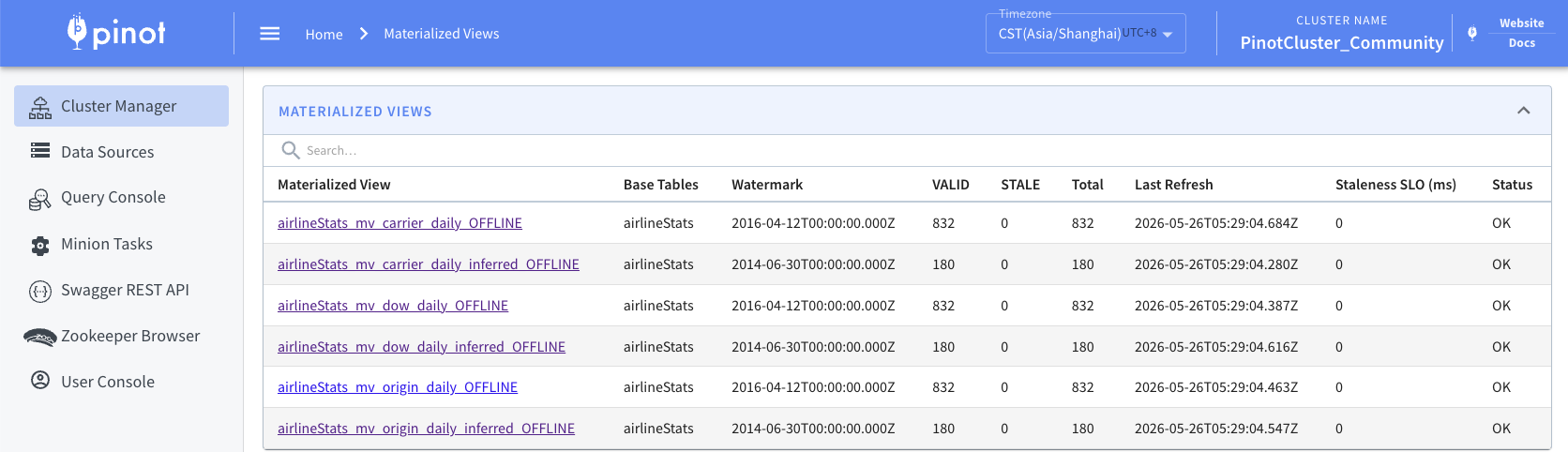
Data Sources view in the Pinot controller UI: each materialized view is a first-class entry alongside regular tables, listed with its base table, freshness state, and last refresh time.

The column list writes itself （Schema Inference）

That third bullet hides most of the actual implementation. When you omit the column list, Pinot derives the MV schema from the AS SELECT projection at DDL-compile time. The query is run through Calcite’s validator against the live cluster catalog, so column typos, wrong arity, multi-source JOINs, and type mismatches all fail as a 400 the moment you submit the DDL — not at the first refresh, and not at the first query.

Each output column then maps to one of three shapes:

The time column — the alias matching the timeColumnName property — is pinned to canonical TIMESTAMP with 1:MILLISECONDS:TIMESTAMP format and 1:MILLISECONDS granularity. The base column can be a millis-epoch LONG; the MV always stores it as TIMESTAMP, and the analyzer separately enforces that bucketTimePeriod divides it cleanly.
Aggregations on the MV allow-list (SUM, MIN, MAX, COUNT, plus the raw-sketch family DISTINCTCOUNTRAWHLL, DISTINCTCOUNTRAWHLLPLUS, DISTINCTCOUNTRAWTHETASKETCH) pick their storage type from a small central catalog (MaterializedViewAggregationCatalog), not from the engine’s surface type. That distinction is load-bearing for sketches: the engine reports STRING for DISTINCTCOUNTRAWHLL(...) because that is the hex-encoded value a SQL client receives, but the MV needs the underlying bytes to re-aggregate. The catalog overrides those three to BYTES so the rewrite path stays correct without the user ever having to think about it.
Everything else — bare columns, scalar transforms, any function not on the allow-list — takes Calcite’s validated type and lands as DIMENSION, NOT NULL, no default.

The few rules the user does have to follow are mechanical: every computed expression needs an AS alias, aliases must be unique, the timeColumnName alias must actually appear in the projection, and SELECT \* is rejected. Anything that needs a non-DIMENSION role, a multi-value column, a custom default, or a non-canonical time-column shape falls back to the explicit column-list form — which we have not yet needed for any of our internal MVs.

Behind the scenes, the compiler turns the DDL into the same (Schema, OFFLINE TableConfig) pair Pinot uses for any offline table, with MV-specific bookkeeping (task.MaterializedViewTask.definedSQL, the resolved Quartz cron) folded into the task config. The watermark — “how far the MV has confirmed coverage” — is intentionally not set by the compiler; it starts at zero and only advances when the scheduler completes its first refresh. That is the explicit handshake that keeps the rewrite engine from picking up an MV that has nothing in it yet.

The rest of the post shows what the engine does the moment this view exists — without the dashboard team changing a single line of SQL.

What runs where

Three Pinot processes coordinate through ZooKeeper. The Controller owns the DDL surface, flips MV partitions to STALE when base-table segments change, and emits refresh tasks. The Broker reads MV metadata at compile time to decide whether to rewrite a user query. The Minion runs the refresh task, builds new segments, and advances the per-partition fingerprint and watermark. Servers execute whichever table the Broker dispatches — unchanged.

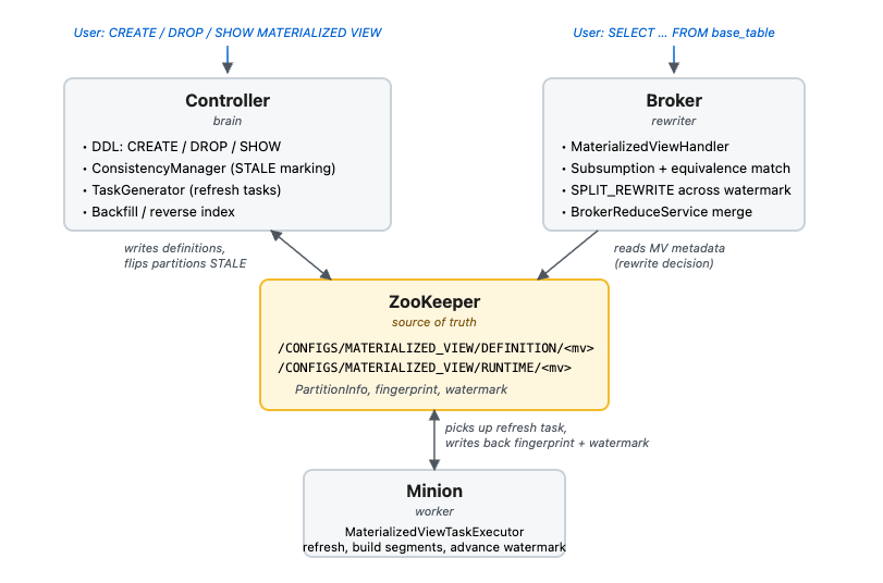
Same SQL, different execution

Take one of our largest fact tables. cdr_events is a Call Detail Record table holding more than ten billion rows across tens of terabytes of storage and 13 months of retention, with tens of millions of new rows landing every day across tens of thousands of customer organizations.

This table sits behind a tenant-facing dashboard with a time-range picker — the user chooses the window. Most stick to the defaults (last 7 or 30 days). But it is entirely normal for less-experienced users to widen the window to 6 months, or to the full 13-month retention, to “see the long trend.” Every one of those clicks is a full table scan over the chosen range.

Here is the actual query behind the dashboard’s “Off-Net Calls” tile:

SELECT DISTINCTCOUNTHLL(correlationid) AS "Off Net"
FROM cdr_events
WHERE on_off_net = 'off_net'
  AND orgid IN ('4***')
  AND callstarttimemillis >= 1771804800000   -- 2026-02-23
  AND callstarttimemillis <= 1774224000000   -- 2026-03-23

Time bounds align with day boundaries here; off-boundary bounds would introduce up to one day of drift per edge.

At a 4-week window for a single tenant, this query scans roughly 150 million rows to compute one number — the count of distinct off-net calls — with the HLL sketch rebuilt from scratch on every replica that touches the request. End-to-end latency: just over one second.

That is for the 4-week default. Widen the window to 6 months and the scan grows to roughly 1 billion rows. Widen it to the full 13-month retention and you are scanning more than 2 billion rows — to render a single tile. Multiply by tens of thousands of tenants refreshing their own dashboards independently, and the cluster overload scenario from earlier is exactly what you get.

Now consider this materialized view:

CREATE MATERIALIZED VIEW cdr_events_daily_dcount AS
SELECT
  DATE_TRUNC('DAY', callstarttimemillis) AS day,
  orgid,
  on_off_net,
  DISTINCTCOUNTRAWHLL(correlationid) AS correlation_id_hll
FROM cdr_events
GROUP BY day, orgid, on_off_net

Three deliberate choices:

The MV stores DISTINCTCOUNTRAWHLL (raw HLL sketch bytes), not the cardinality number. Numbers cannot be safely combined later; sketches can.
The grain is day × orgid × on_off_net — every dimension the dashboard can filter or group by.
The partition column is day, so any query’s time range can be aligned to whole-partition boundaries.

With this MV in place, Pinot’s rewrite engine transforms the user’s query into:

SELECT DISTINCTCOUNTHLL(correlation_id_hll) AS "Off Net"
FROM cdr_events_daily_dcount
WHERE on_off_net = 'off_net'
  AND orgid IN ('4***')
  AND day >= 1771804800000
  AND day <= 1774224000000

The output is identical. The work to compute it is not. The rewritten query reads 29 rows instead of roughly 150 million — one pre-computed sketch per day, merged in microseconds. End-to-end latency drops to roughly 200 ms — a ~5× user-side speedup. And the long-window cases scale gracefully: at 6 months, the cluster reads 180 rows instead of ~1 billion; at 13 months, around 400 rows instead of more than 2 billion. The cost of “show me a longer view” stops being scary.

The MV itself is small. Across the full set of active orgs, two on_off_net values, and roughly 400 days of retention, it produces on the order of tens of millions of rows / tens of GB — two orders of magnitude smaller than the source table. The cost of remembering is a small fraction of the cost of recomputing.

The bigger win is not the latency

A 5× speedup on a single dashboard query is the visible part of the story. The invisible part is what matters more to operators: the cluster scanned more than five million times fewer rows for this one query.

Fewer rows scanned means less segment data loaded off disk, less heap churn while building HLL sketches, less CPU on filter and projection, less network traffic across replicas. Every byte the cluster does not have to read is a byte not competing with ingestion throughput, concurrent queries, or background compactions.

These savings translate directly into the resources that govern cluster stability. For a query of this class, memory pressure drops by roughly 5× and CPU consumption by roughly 20× — direct consequences of the I/O collapse you just saw. Per-query resource attribution for MV-rewritten queries is still maturing in our observability stack, so we are not pinning these numbers to a decimal point yet — but the order of magnitude is hard to miss.

Users get snappier dashboards. Operators get a quieter cluster. That double win — better user experience and better cluster stability from the same change — is the reason this work exists.

How the engine actually finds the view

When the user query arrives, the rewrite engine walks five quick steps:

Parse and identify the query shape: aggregation function (DISTINCTCOUNTHLL), filter columns (on_off_net, orgid, time), no GROUP BY.
Pull MV candidates from MaterializedViewMetadataCache for the source table.
Check aggregation subsumption via AggregationEquivalenceRegistry. The user’s DISTINCTCOUNTHLL matches SketchMergeEquivalence("DISTINCTCOUNTHLL", "DISTINCTCOUNTRAWHLL", "DISTINCTCOUNTHLL") — meaning the MV’s raw HLL bytes can be merged into the user’s cardinality result.
Align the time range via MaterializedViewTimeExpression. The user’s callstarttimemillis predicate is rewritten to reference the MV’s day bucket column, with the epoch-ms literals carried over verbatim.
Emit the rewritten plan — same SQL surface to the user, completely different physical execution.

No code change on the dashboard side. No new pipeline. One DDL statement at MV creation time, and from that moment forward, every qualifying query takes the cheap path automatically.

How the view earns trust

A fast wrong answer is worse than a slow right one. The hardest engineering problem in any materialized view system is not building the views — it is deciding, at query time, when a given MV partition is safe to read. Pinot’s MV layer makes that decision explicit, per partition, with a small state machine that both the refresh path and the read path can reason about.

Before the state machine itself, the picture: an MV is laid out as a fixed-width grid of partitions over the base table’s timeline, with each bucket fed by whichever base segments happen to fall into its window. The bucketTimePeriod knob from the DDL is exactly what fixes the grid’s width — and every freshness check, refresh task, and rewrite decision in the rest of this section reduces to per-bucket reasoning over that grid.

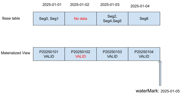
The MV’s bucket grid laid over the base table’s segment timeline. Each MV bucket aggregates the base segments whose data falls into its window; the bucketTimePeriod knob from the DDL is what fixes the grid’s width.

Per-partition freshness, not all-or-nothing

Every MV is sliced into time buckets of fixed width, and for each bucket Pinot stores a small PartitionInfo record in ZooKeeper:

bucket = 2026-02-23  →  { state: VALID, segmentCount: 47, crc: 0x5e3a…, lastRefreshTime: 1771823412000 }
bucket = 2026-03-23  →  { state: STALE, segmentCount: 12, crc: 0x9b1f…, lastRefreshTime: 1773002145000 }

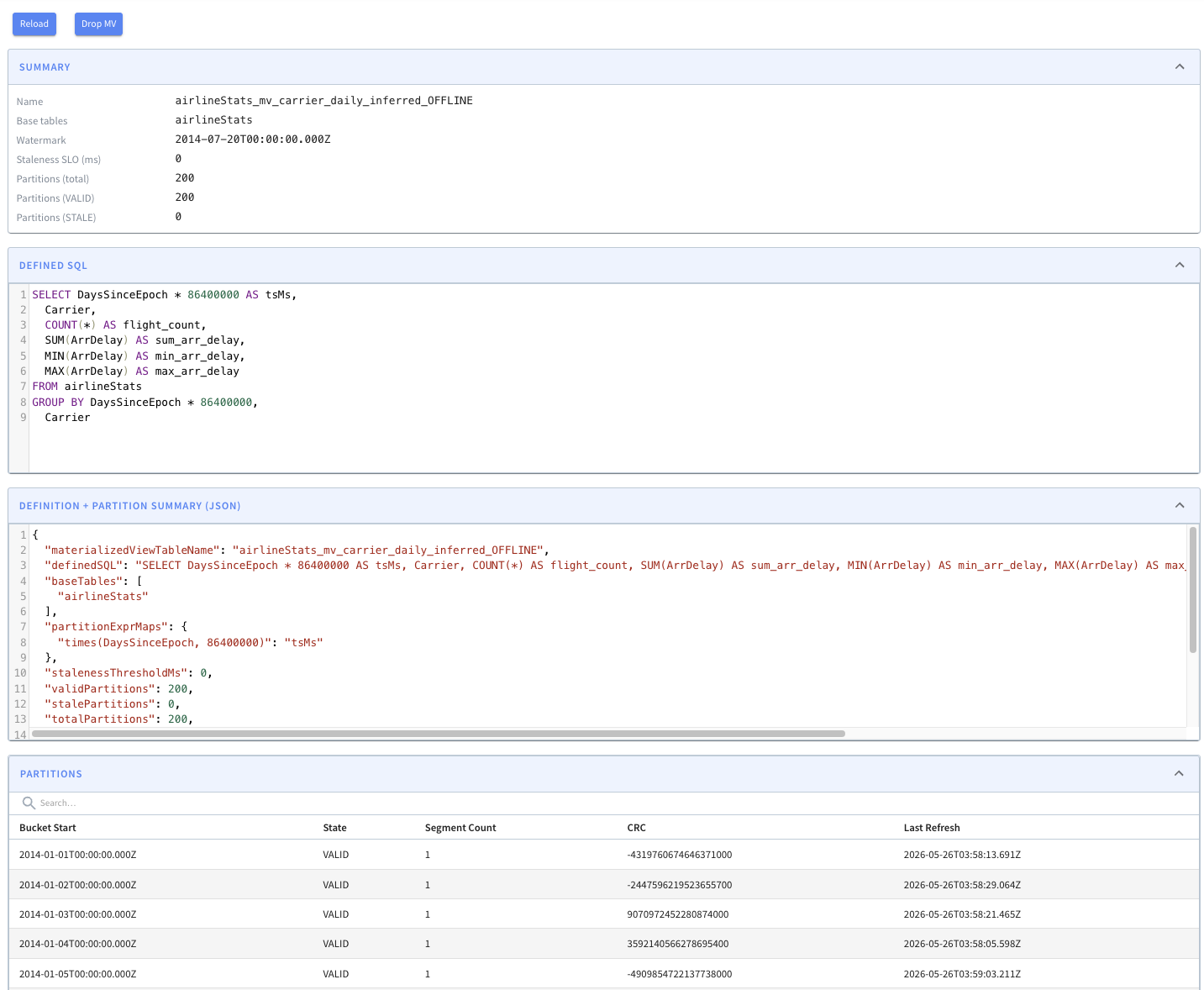
MV detail page in the Pinot controller UI: per-bucket VALID / STALE state, the MV’s watermarkMs, and the last refresh time are exposed to operators directly — the same data the rewrite engine reads at compile time to decide whether to redirect a query.

Freshness is a property of each bucket, not of the whole view. A user asking about February does not care that March is in the middle of a refresh. The PartitionFingerprint — segment count plus a CRC sum across the base segments that fed the bucket — is what makes the freshness check robust: if a base segment is swapped for a different one at the same count, the count alone would not notice, but the CRC will.

When a base-table segment is added, replaced, or deleted, MaterializedViewConsistencyManager picks up the ZK event, debounces for five seconds to coalesce bulk ingestion bursts, intersects the affected time range with each MV’s bucket grid, and flips overlapping buckets to STALE. It is event-driven, not polled — idle clusters do no work.

Refresh without blocking reads

A scheduler (the Generator) periodically scans for STALE buckets. Before submitting a refresh task it re-reads the current base-segment fingerprint and compares it to the stored baseline; if they match, the stale marking was a false positive (a segment churn that did not actually change data) and the bucket is quietly returned to VALID without recomputation. Real changes go on to the Executor, which materializes the bucket, writes the new fingerprint, flips state back to VALID, and advances the MV’s watermarkMs — “everything strictly below this timestamp has confirmed coverage.”

That watermark is what closes the loop with the query path. When a user’s time range crosses it, the broker switches into ExecutionMode.SPLIT*REWRITE:`` the MV serves the cold half (ts < watermarkMs), the base table serves the hot half (ts >= watermarkMs), and BrokerReduceService` merges both sides using the user’s original query as the merge key. The user gets the latest ingested data _and* the pre-aggregation speedup on the cold half — they never wait for a refresh to finish.

Bucket-level consistency is a deliberate choice. Analytics dashboards look at completed time buckets, not “as of two seconds ago,” and the bucket boundary maps cleanly onto a freshness contract a human can reason about. For workloads that need stricter freshness, operators can lower stalenessThresholdMs (the rewrite engine will skip an MV whose watermarkMs falls outside the SLO) or set rewriteEnabled=false to take the MV out of the rewrite path entirely. Schema changes, partial uploads, controller failover, and cold-start — the cases that would silently corrupt a less careful system — are each caught by an explicit gate before any MV row is returned.

What it bought us

Pinot’s MV layer hasn’t been in production long enough to publish quarter-over-quarter savings curves, but the shape of what it changes is already visible at three different altitudes.

Cluster stability. When a stable query pattern hits the same fact table hundreds of times an hour from different dashboards, the rewrite engine collapses that pattern down to a handful of pre-aggregated rows. Less data read from disk, less scan work across replicas, less heap pressure during sketch construction. The cluster-overload pattern from earlier — where unrelated tenants pile onto the same expensive aggregation — becomes much harder to trigger.

Query latency. A user query that hits an MV reads a row count proportional to its time range in buckets, not to the source table’s row count. The “what if I widen the date picker to a year” case — the one users used to learn to avoid — flattens out. Dashboards stay snappy at windows where they used to crawl.

One less pipeline. The external daily-aggregate ETL pattern from earlier collapses into a single CREATE MATERIALIZED VIEW statement that the cluster owns end-to-end. No second schedule, no second failure mode, no second source of truth.

What’s next

Two pieces of work are in active design.

Hybrid table support. MVs today are built over OFFLINE source tables, which fits batch-ingested fact tables well but excludes any table whose freshest data lives in a realtime segment. The roadmap here is to extend MV bookkeeping — partition fingerprints, the consistency manager, the watermark contract — to hybrid tables, so a realtime-backed dashboard can sit on the same MV layer the offline tables already do today. The freshness state machine from the previous section is designed to carry this extension without changing its core contract.

Multi-Stage Engine (MSE) query support. Transparent rewrite today runs on Pinot’s Single-Stage Engine. The next milestone is to let MSE queries read MVs directly — users referencing the MV table by name in an MSE query plan — before the more invasive step of teaching MSE planning to find the right MV automatically. Direct access first, transparent rewrite second.

Try it

The Materialized View feature is merged into Apache Pinot. The code lives under the pinot-materialized-view module and ships with a self-contained quickstart that builds the base table, creates an MV, runs the minion refresh task, and validates the rewrite end-to-end:

bin/pinot-admin.sh QuickStart -type MATERIALIZED_VIEW

Transparent rewrite is gated behind a broker switch — pinot.broker.query.enable.materialized.view.rewrite=true — so it can be enabled per cluster as teams evaluate it on their own workloads. Full reference — supported aggregations, source-table requirements, REST endpoints, and the Data Explorer UI for inspecting MV state — lives in the Apache Pinot materialized views documentation.

If your workload looks like the ones in this post, we would love to hear how it lands.

More details and updated information about Materialized Views in Apache Pinot in the Docs